Why this matters: Pricing in the real estate market moves between extremes, juxtaposed within short-term seasonal and long-term business cycles. Readily available studies allow real estate agents to anticipate the effects of the approaching phase in the pricing cycle, which is never static. With an awareness of changing conditions, distractions and foreseeable instability, these agents advise clients on the economic outlook for pricing.
The mean price trendline presents the inherent value to which all property pricing returns, a magnetic-like vertical pull following each eventual peak and bottom in pricing during a business cycle.
Waiting for the fall
Home prices since 2012 through the pandemic period became far removed from the mean price trendline. In response, fewer homebuyers are willing to pay asking prices which rise noticeably faster than their incomes. Without an offsetting reduction in mortgage rates, as took place in the three decades before 2012, recessions occur in short time spans.
Record-low interest rates during the pandemic years of 2020 and 2021 temporarily relieved the homebuyer purchasing power crunch produced by rising FRM rates. The artificially low mortgage rates in the pandemic contributed to a frenzy in 2021 of pandemic-era home buying, which drove pricing 1/3rd higher than in 2019, when it was already distorted. However, interest rates quickly reversed course coming into 2022, removing support for a home seller’s prior year asking price.
As properties became overpriced for rising FRM rates, home sales volume began to decline rapidly in Q2 2022. Prices began a premature decline just three months later. This abrupt shift in pricing was unusually fast coming, as pricing expectations tend to be stickier, taking nine to twelve months to follow a decline in sales volume.
Considering the pandemic tsunami of price supports, the level of damage left in the wake of the pandemic retreat was initially severe. Pricing was left, with nothing to stick to but seller illusions of past pricing. However, unusually low levels of inventory for sale kept prices plateaued during 2023 and 2024 in spite of a general buyer withdrawal.
In 2025, the drag on new construction from rising building costs, due to trade wars combined with immigrant issues, further adversely affected the home sales volume. Meanwhile, buyer caution about declining jobs and rising mortgage rates lowered buyer willingness to make offers. As buyers stepped back, property sales volume declined further. The result was a 1/3rd increase year over year in inventory for sale by mid-2025.
firsttuesday forecasts a continuation of falling home prices in 2025, dropping to cross over the mean price trendline before a bottom appears in pricing, likely in 2027. Pricing below the mean price trendline is not expected to return to cross over the mean price trendline for two or three years after initially hitting bottom prices.
Bottom pricing is brought about as a stop to property price decline by the first wave of buyers to arrive – speculators (flippers) and buy-to-let investors acquiring property they perceive as priced cheap, generally below the mean price trendline.
As prices form a bottom over 12 to 18 months of initial investor and flipper acquisitions, inventory for sale starts to thin and prices stabilize before starting a slow rise. Only then do end-user buyers sense the decline in pricing is over and begin their return which drives prices toward the mean price trendline. The timeline before prices return to the mean price trendline, but not the real estate sales events, is complicated by global-wide events.
Updated July 17, 2025.
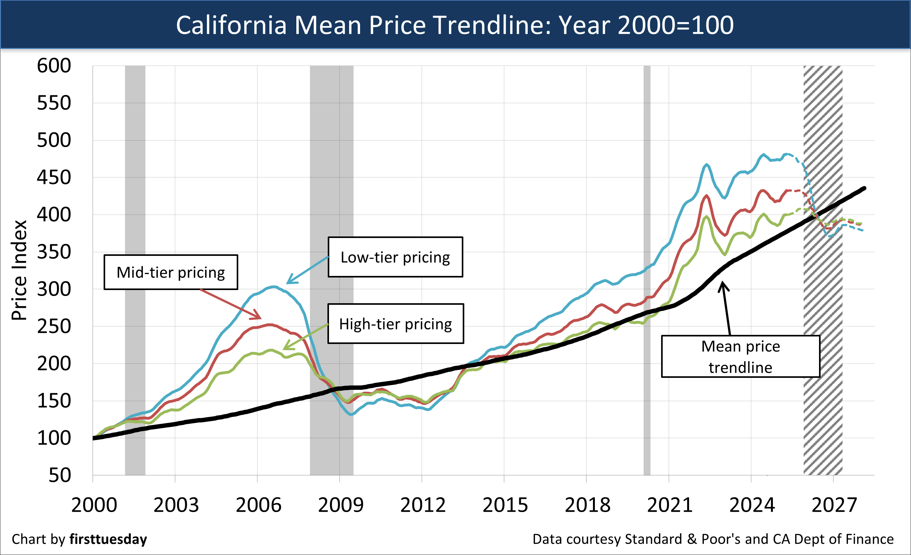
Chart update 8/14/25
The blue, red and green lines track sales price fluctuations within the three single family residence (SFR) tiers in California’s largest cities. The dashed lines are firsttuesday’s home price forecast. The black line is the mean price trendline. The mean price trendline represents the historical equilibrium level to which property prices cyclically return.
Grey bars indicate periods of recession, with the grey dashed bar firsttuesday’s forecast for the next recession, currently underway.
Property prices sellers receive from buyers rise and fall as though tethered to the mean price trendline. Property price movement crosses the mean price trendline twice during each business cycle as prices rise and recede like a tide.
A comparison of contemporary prices with the mean price trendline tells us how far today’s prices deviate from the long-term norm and forecasts price levels likely to develop in the years immediately ahead.
The hazardous intersection of price illusion and reality
My house is worth how much? Owners can quickly tell you the price of their home, as do seller brokers. But sellers and buyers have no knowledge of its current value. The market price of a capital asset – real estate of any type – is in constant flux in response to today’s market conditions and the demographics of its buyers and sellers. The market price is readily known to brokers and agents active in the market, and in turn their clients as advised.
But does a way exist to measure a property’s innate dollar value over time?
Indeed there is — by referencing the mean price trendline. The trendline contains the wisdom of long-term running averages, here based on wage inflation. Consumers are anchored to their income and, in turn, what their income will buy, not what sellers want for their property. Critically, a trendline eliminates the “noise” of short-term year-to-year asset pricing, especially boisterous during peak and bottom years in business cycles of extended duration.
Boom periods are times of economic plenty – excess earnings from increased employment ready to spend and used to borrow and leverage a wage earner into a higher living standard than otherwise. Sellers of property happily embrace these conditions as prices soak up the extra cash to produce excess profits on a sale. Soon builders rush in to normalize, and sometimes distort, availability of inventory and pick up a share of the additional homebuyers, and with luck, profits.
Boom-time markets, flush with cash and rising real estate prices, appear untethered from historical price trends. Market advisors declare a new paradigm, which never comes about. The following fallout is financially damaging for mortgage-funded buyers who acquired a home within two years before and after peak prices. During these short-lived virtuous cycles within a generic business cycle, sellers and seller agents dominate negotiations in real estate transactions, adding further distortions for buyers.
The momentum and volatility of boom times appears strong on balance sheets for property owners. But they rarely last long. Without a sale or refinancing to realize the market price during the peak of a boom they are simply “paper profits” no longer supported by the evolving market value of property.
Eventually, sales volume evaporates, prices slip and buyers take note by initially just watching the (in)action – except to observe the drop in pricing. The boom becomes a bust, commencing the recessionary process known as the vicious cycle.
At some point in a recessionary period, jobs and other favorable economic conditions return. In time, buyers are encouraged to willingly make offers and acquire property. Property sales momentum picks up. Prices rise again and crossover to exceed the mean price trendline – a return of the virtuous cycle, the recovery portion of a garden variety business cycle.
Neither a boom nor a bust is sustainable long term. They are, by their nature, short-term divergences. As such, they’re unfit for measuring long-term value for any parcel of real estate. However, as the booms and busts create their peaks and valleys in seller pricing, a durable long-term trend line in pricing remains– a property’s inherent dollar value.
When the mean price line is viewed alongside the lines for home prices paid by buyers, the wisdom of the crowd becomes clear as shown in the above chart.
The mean price trendline: Consumer inflation plus
Through the turmoil of booms and busts, prices repeatedly return to the mean price. Mean pricing is primarily dictated by:
- the path of consumer inflation, as measured by the Consumer Price Index (CPI); plus
- a California premium of, say, 1.5% annually.
Consumer inflation is inextricably tied to wages from jobs to fuel consumer spending. No job, no spending sufficient to support pricing.
How does CPI affect home price trends? There are two major ways:
- The CPI affects the fundamental measure of a property’s value: the replacement cost of land, materials and labor as setting value.
- The CPI reflects changes in spending on consumer goods and services. To compensate for employee pay demands due to their increased costs of living, employers typically increase staff income in step with the CPI, the COLA pay raise. As a potential homebuyer’s income increases, so does their purchasing power through their capacity to borrow greater sums of money, assuming no increase in FRM rates.
The California premium accounts for value added to its real estate by the allure of its geography, business opportunities, infrastructure, educators, cultural diversity and political stability. This is the stuff which makes California’s economy the fourth largest in the world with only a 40-million population. Breathtaking, when you think about it.
Thus, the mean price trendline represents the long-term value of property at any point in time, as adjusted for consumer inflation plus an annual California premium of around 1.5%.
An enlarged picture of California price movements is observed by reviewing the disparity – spread – in the velocity of price movement between low-, mid-, and high-tier sales. Pricing in these three tiers vary based upon our population’s wildly divergent financial capacity to buy a home.
To best present a statewide view of price movement, we look to California’s three largest metropolitan areas: Los Angeles, San Francisco and San Diego. Each area’s sales prices are then segmented into three price tiers; low, mid and high with 1/3rd of sales volume in each.
Homes sales are classified by price range to display a clear picture of how prices move in each tier of the market over time. Each tier’s pricing accelerates and decelerates at significantly different paces. Typically, pricing in the high-tier does not fluctuate as much as in the mid- and low-tiers, with low-tier pricing being the most volatile.
Related article:
The crossover moments are twice in a cycle
Home price movement between the zenith at peak prices in a boom and rock bottom prices in a bust create crossover moments as pricing drops below and rises above the mean price trendline. This is akin to leaving a seller market and entering a buyer market or leaving a buyer market and entering a seller market in a pricing sphere.
A seller market is a period when prices trend higher, further rising above the mean price trendline. During this period, sellers realize excess pricing on the sale of their homes. At the same time, families buying a home in this period overpay to become homeowners rather than tenants. The reverse financial experience for buyers exists when prices remain near or below the mean price trendline.
Related article:
Buyer Purchasing Power Index (BPPI) hints at rising as home price adjustment sets in
As evidenced by the past
A quick review of the recent past is needed to move your understanding forward.
Home prices in the late 1980s reverted to the mean price trendline after the July 1990-March 1991 recession. Between 1991 and 1999, prices were depressed, and the cost of property was low, from a historical perspective. Accordingly, prices dipped below the trendline during this period, a buyer market.
Prices began to rise in 1997, growing to cross over the mean price trendline in 2000. At that time, the mean price trendline index and California Consumer Inflation index were, for a fleeting moment, at the same price point: the crossover moment.
After crossing the mean price trendline in 2000, real estate prices were allowed to begin a skyward trajectory. The 2001 recession was short-lived without a price correction, due to excessive monetary and fiscal stimulus reaction to September 11, 2001.
As a result, the price of homes froze in 2001 at their artificially elevated, pre-recession peak. Instead of reverting to the mean price trendline, prices leveled out.
After 2001, prices continued to rise going into a steep trajectory fueled by an influx of money from federal fiscal and bank deregulatory activity. This period is now known as the Millennium Boom. Real estate prices peaked going into 2006. Then with the onset of the Great Recession began their precipitous decline – back to cross over the mean price trendline, to bottom in the 2009 to 2011 period before rising again.
The mean price trendline forecast
Home prices continued to stall in all tiers across Los Angeles, San Francisco and San Diego during April 2025, the result of buyer unwillingness at a time of reduced purchasing power.
Since the same time last year, San Diego and San Francisco hovered at 1% growth in all tiers except San Francisco’s mid-tier, dipping down 2%. Los Angeles saw the most rise, only making a 3% growth across the low- and mid-tier price points.
Home prices surpassed their May 2022 peak in San Diego and Los Angeles, ranging from 3% to 6% growth across the three tiers in San Diego and rising 6% to 7% during the same time in Los Angeles.
In contrast, San Francisco’s tiers shrank 8% overall. Keep in mind that pricing of the most expensive homes forecasts future trends across all tiers. Expensive homes are both the first to rise and the first to fall, with San Diego and Los Angeles expected to follow San Francisco’s downward trend.
With such a disappointing 2025 spring bounce due to consistently high mortgage interest rates, watch for inventory to build up to further reduce pricing.
This price decrease will first be resisted by sellers’ stubbornness, known as the sticky pricing phenomenon. Many sellers in a devalued real estate market of resetting prices hesitate to sell at current market value as prices trend even lower.
However, the timeline is complicated by government trade wars, reduction of the necessary migratory labor force, international turmoil, and vicissitudes of uncertain government action.
Adaptable agents pursue long-term and recession-proof occupations of income property management, residential income sales and MLO financing of home sales. These are each consistent moneymakers as they survive turmoil. People always need shelter and someone to arrange it.
Related article:


Great info. Thanks so much for sharing. I also found the same conclusion by looking at trend lines on CPI data using FRED chart.
Thanks for a lot of good analysis. However household income is probably a better basis for comparison than the CPI. In some areas like Silicon Valley incomes are increasing faster than in other areas and faster than inflation. And incomes do not automatically keep up with the CPI as people in rustbelt states know.
Valuable analysis . I loved the information , Does someone know if I can get a sample CAA Form 3.0-R example to fill out ?
Oren,
Thank you for your inquiry. RPI publishes an Application To Rent Form 553. You can download the form here or from our forms download page.
Regards,
Editorial Staff
Thanks for the many fine first tuesday articles. You folks are extraordinary. I’m no longer a CA broker, no longer even living in CA, but I read you religiously and do share, with credit.
Dear Richard,
Absolutely. You are encouraged to share this information and all other articles, with credit given to first tuesday Journal Online.
Also, if you are not already a subscriber, feel free to sign up for our weekly newsletter which includes statistical updates, FARM letters and other information tailored for you to share with clients. Sign up here.
Regards,
Editorial Staff
As a broker, I am amazed in the amount of quality information you give away. This is information every investor
in Real Estate should see as to what the future might hold.
Do I have your permission to share this information with my clients?
Richard Guess
I think that the real estate market has much further down to go beyond 10%-15% in price and in market psychology. If you look at the chart by Dr Jean-Paul Rodrigue’s, economist at Hofstra University, of the main stages of a bubble it is very close to the chart you show of CA home prices, up to the present. The bubble ends with the current blow off Stage. The last part involves capitulation and then at the bottom despair. Were not there yet. We have been to Ca real estate will never go down. The opposite extreme is it will never go up. Not even close to there yet. There is a consensus now that the bottom is in sight, not capitulation and not despair.
Also from the chart of the Bubble Theory, the bottom occurs below where the bubble started. That would bring prices below 1997 prices. Such a move would be certain to elicit capitulation and despair.
The Bubble Theory Chart is available online in a Financial Times article about the British real estate bubble: http://ftalphaville.ft.com/blog/2009/03/12/53476/bubble-theory-and-uk-housing
A drop to the mean price trendline would be about a 33% drop (mid tier 330 to 210).