This article explains how interest rates impact buyer purchasing power and home prices.
The driving force in real estate pricing
Buyer purchasing power is the driving force behind real estate pricing.
On one side of the pricing scale sits the buyer with some down payment money. On the other is the seller with a property. Between them sits the all-powerful lender with funds necessary to close the transaction. As with a seesaw, the lender’s mortgage rate moves the pricing up and down.
This chart displays the Buyer Purchasing Power Index (BPPI). This index measures the year-over-year change in the amount of mortgage money available to a buyer based on average gross income. It varies based on the interest rate charged for a 30-year fixed rate mortgage (FRM).

An index number of zero translates to no year-over-year change in the amount a buyer can borrow. A positive index number, say 5, means the buyer can borrow 5% more money this year than one year earlier. The index is based on today’s incomes.
Finally, a negative index number translates to a reduced amount of mortgage funds available to a buyer compared to one year earlier.
At the end of 2022, the BPPI was -31. This figure tells us a homebuyer with the same income today is able to borrow 31% less purchase-assist mortgage money than a year ago when mortgage interest rates were still near historic lows.
Related article:
Press Release: Buyer Purchasing Power Index ends 2022 31% below a year earlier
Mortgage funds available, but limited by rates and buyer’s income
This chart contrasts the average 30-year FRM rate with the corresponding mortgage funds available, in today’s dollars. From the 1980s through 2012, interest rates generally decreased, resulting in more funds available to buyers each year. Since 2012, mortgage rates have generally increased.
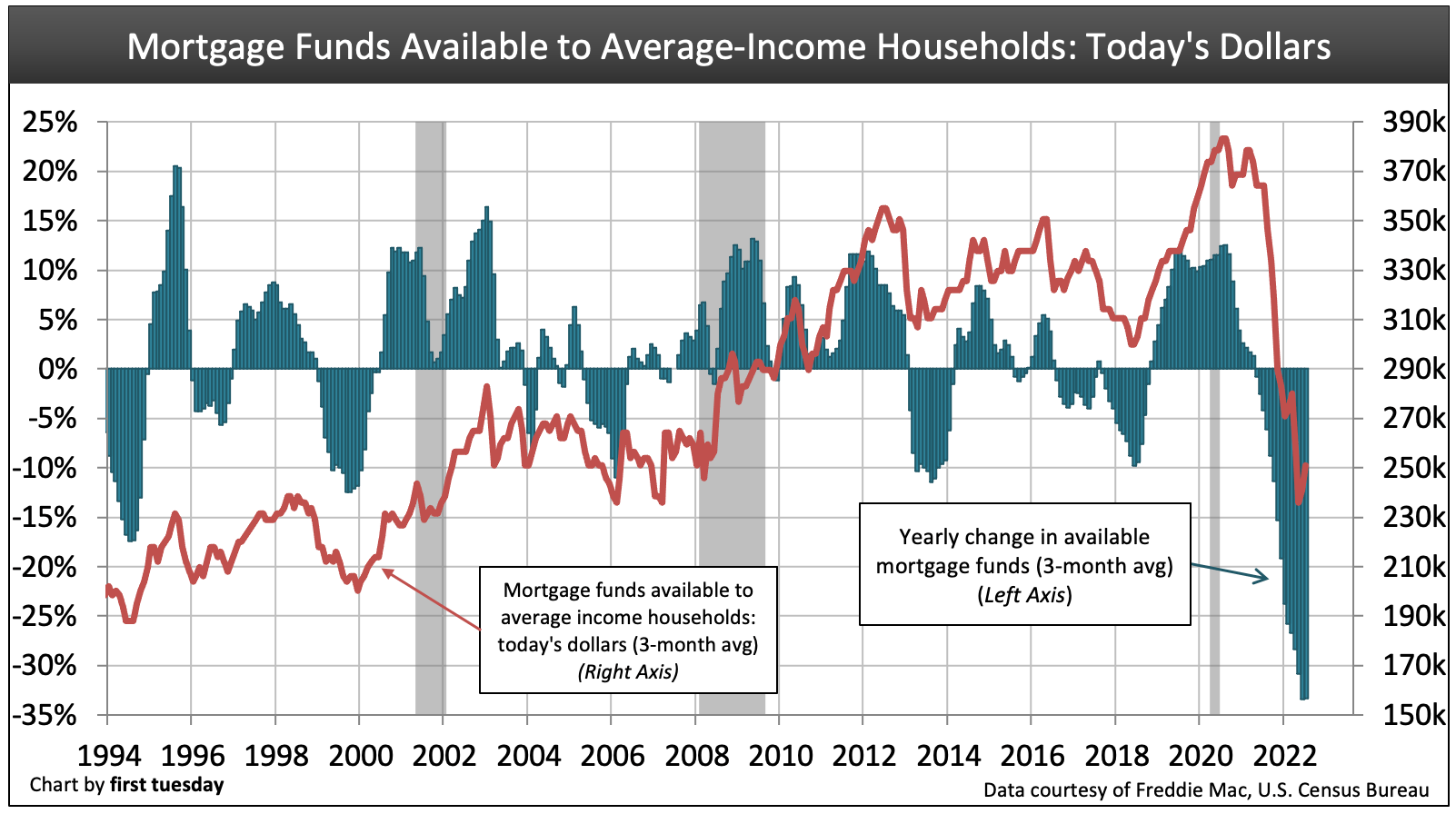
The mortgage funds available to a buyer from year to year are depicted by the solid line on the chart above. These amounts are in today’s dollars and are based on the mortgage amount an average income earner in California qualifies to borrow.
Payments are set at 31% of gross income (before withholdings), as required for qualified consumer mortgages.
What appears is a purchasing power drop of roughly $150,000 in the amount an average buyer can borrow with the same income over the past year — due solely to 2022’s interest rate jump.
The yearly change in available mortgage funds (shaded bars) depicts the percentage change in mortgage funds available to a buyer compared to one year earlier. Mortgage funding changes in lockstep amount as interest rates rise and fall. The higher the shaded bar, the higher the mortgage amount a buyer will qualify for compared to the previous year using today’s pay.
In the coming decade, the annual BPPI figure will generally remain negative due to continually rising interest rates, a turnaround of long-term interest rate movement which began in 2012. The impact to homebuyer mortgage funding has been devastating — and the inevitable shockwave to home prices arrived in the second half of 2022, pushing prices to rapidly implode.
However, this decrease will be slightly offset by an annual increase in the wages of homebuyers.
The lender determines the buyer’s mortgage amount
Each buyer has a maximum price they can pay to purchase property. This maximum price depends on:
- the buyer’s down payment; and
- the mortgage funds they qualify to borrow from a lender.
The amount of mortgage funds a buyer can borrow is based on two factors:
- the buyer’s income, which adjusts annually at the rate of inflation; and
- current mortgage rates, which change constantly.
Lenders know buyers are less likely to default if they allocate no more than 31% of their monthly gross income to their monthly mortgage payment. Accordingly, mortgage lenders refuse (as mandated) to lend more money than the buyer can repay at that 31% gross income ratio, amortized over 30 years.
The buyer’s income and mortgage control the seller’s price
On the other hand, sellers seek the highest possible sales price they can get from a buyer whose standard of living is typical for the location. The sales price of all homes sold within each pricing tier cannot on average exceed the purchasing power of buyers shopping in that tier.
When all sellers within a tier hold out for above-market prices, buyers for that tier of property will eventually be unable to buy. Thus, buyers control the price sellers will receive, based primarily on mortgage funds available at current interest rates.
Sellers of any type of asset have received greater and greater prices over the past 20 years driven primarily by a continuous drop in interest rates (a Fed activity historically called the Greenspan put).
However, the pricing trend has reversed, moving out of the zero lower bound interest rate regime we left in 2012. And the downward pressure on prices will continue for a long time as interest rates are unlikely to drop for the next couple of decades — except temporarily during Fed-engineered business recessions.
Rates hovered near zero from 2009-2015 and again in 2020 — and while a rate of zero was too high to stimulate the economy, the Fed (unlike some countries) was unwilling to go negative. Expect rates to trend upward over the next 20 years (except during recessions).
As mortgage rates rise, the maximum price a buyer can pay for a home declines since the amount they are able to borrow declines.
The static 31% debt-to-income (DTI) ratio is set for buyers needing a mortgage. Going forward, buyer income will rise annually based on consumer inflation of around 2%. This inflation figure has been typical for nearly two decades — with the rapid inflation of 2022 the big exception. However, wages have not kept up with consumer inflation, much less asset inflation (think homes) over the past 15 years.
Related article:
Reading the charts
As interest rates rise, the interest portion for the same monthly amount of payment on a new mortgage increases.
The result is a reduction in the portion of each payment that goes toward amortizing mortgage principal. In turn, the amount of principal the same monthly payment will amortize is smaller. The smaller the principal mortgage amount the buyer can borrow, the less price sellers can get from buyers. It is axiomatic.
Consider California’s average monthly household income of $5,016. At 31% of this monthly income, the maximum mortgage — and principal, interest, taxes and any impounds (PITI) — payment the average homebuyer with less than 20% down payment can qualify for is $1,155. This amount includes PITI the buyer pays to the mortgage holder.
Thus, the amount of money available monthly to repay the mortgage for a new home (the principal payment) changes from week to week as interest rates rise and fall. The rates used on the charts are for a 30-year FRM.
Related article:
Historical examples
Consider the significance of the one-year rate differential in the following historical examples:
- 2003: Mortgage rates were too low during this period, an aberration in rates due to the Fed’s overreaction to the 9/11 attacks. The Fed kept rates low, instead of allowing the 2001 recession to work its price-reduction magic. Due to lower rates, buyers were able to borrow much more than they were able to a year or two earlier.This led to a spike in buyer purchasing power. Sellers and their agents recognized the increase in mortgage amounts buyers qualified to borrow, and began demanding higher prices. Add to this math the financial accelerator effect of ever larger mortgage amounts from all types of lenders driving home resale prices. Thus, lenders accepted these homes as collateral at ever greater valuations artificially driven further up by nothing more than increased mortgage amounts. Lenders foolishly accepted that condition.
- 2004 and beginning of 2005: FRM rates flattened, causing buyer purchasing power to stabilize. However, property prices were rising. To compensate for this mixed price/lending condition, lenders, homebuyers and speculators resorted en masse to adjustable rate mortgages (ARMs). ARMs allowed lenders to mask the amount of future payments with low up-front rates, called teaser rates, and interest only payments (or less as with negative amortization).
With ARMs, the borrower qualifies for greater mortgage amounts than available by taking out an FRM. However, when those teaser rates adjust upwards, as they do, the borrower cannot repay at the higher interest rate, and sells or defaults.
- Mid-2005: Sales volume reached its peak while prices continued to rise. The diminishing numbers of buyers turned to option-ARMs and alternative A-paper mortgages (Alt-As), also called liar loans, to meet the prices sought by sellers.
- 2006: Sales prices peaked early in the year. Home prices began a decline from their artificially inflated status. Buyers and their agents began setting prices by applying fundamentals related to the real world as competitive bidding disappeared. These fundamentals factored in the replacement cost of land and improvements, and the income approach for setting value. As prices declined, speculators temporarily slipped away from participating in the market, except to dump property and recover cash.
- 2009: The Fed lowered interest rates essentially to zero. The rise in buyer purchasing power seen in 2009 and government stimulus produced the classic dead cat bounce inherent in all recessionary drops. Due to the Great Recession and financial crisis, mortgage rates were dramatically lowered by the lender of last resort — the Fed — as they via the bond market indirectly funded all newly originated home mortgages for the next few years.
This Fed activity provided all the mortgage financing needed by buyers with down payments as little as 3.5%. Governments provided subsidies to stimulate buyers until mid-2010. Unfortunately, reduced rates and down payment amounts also attracted troublesome speculators as flippers depleting inventories. All this again drove prices of low-tier housing to unsustainable levels going into 2010.
The Federal Housing Administration (FHA) contributed to this mini-frenzy by eliminating the 90-day investor holding period through 2014. Flipper activity increased rapidly, interfering with the organic sales recovery at the expense of sellers, end-user homebuyers and the real estate market.
Little rate changes make a big difference
Consider a buyer whose gross annual income ($58,000) allows them to make a monthly payment of $1,500.
The $1,500 monthly payment qualifies them for the following mortgage amounts on an FRM:
| Interest rate | Mortgage amount |
| 4.0% | $314,000 |
| 4.5% | $295,800 |
| 5.0% | $279,200 |
| 5.5% | $264,000 |
| 6.0% | $250,000 |
| 6.5% | $237,100 |
| 7.0% | $225,300 |
| 7.5% | $214,400 |
When the interest rate fluctuates so much as half a percentage point, the mortgage amount changes by thousands. All buyers are subject to the same relative reduction in their mortgages on a rate increase. Thus, sellers as a whole need to accept a lesser price if they are to sell and the market maintain the same pace of sales volume that existed prior to the rate hike.
Sellers’ sticky price delusion
Other factors weigh in to change the dynamics of this formula.
Sellers, by nature, are culturally susceptible to the age-old real estate phenomenon of sticky prices during recessionary periods. Sellers generally are uninformed about pricing properties in the real estate market. Instead, they believe that they need to get more for their property than the neighbor did down the street, whether it sold last year or the year before.
This sticky price phenomenon leads to a seller’s delayed response in properly pricing their property to keep pace with the market. As a result, when mortgage rates rise, the real estate market moves toward a stand-still, a solstice moment. Soon, sellers and their agents belatedly conclude prices need to be dropped to sell and return sales volume to its norm.
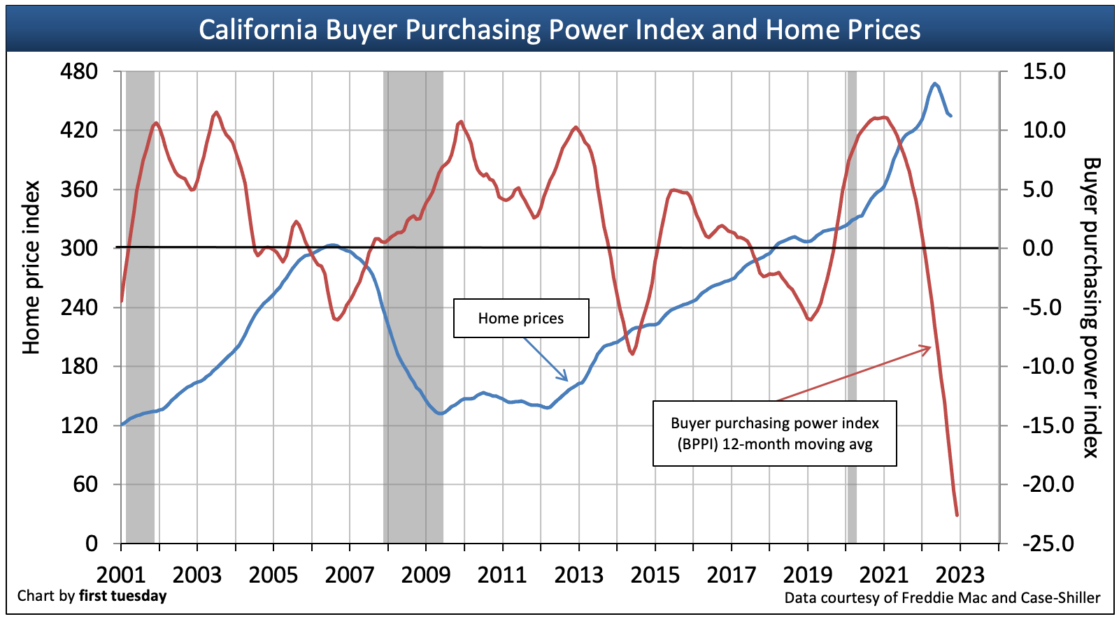
Here, picture the influence of the BPPI (the red line) on home price movement (the blue line). While BPPI went negative in 2006, home prices quickly fell back. When the BPPI next went negative in 2014 and again in 2019, home prices did not fall back, but rather flattened out. Insufficient housing available to meet demand in California and an expanding economy contributed to the continual positive movement in home prices during 2012, ending in early 2022.
Beginning in January 2022, the BPPI rapidly went negative, hitting a low of -31 at the end of 2022. With significantly less mortgage funds available, buyers began making offers at lower prices in the second half 2022, with prices still falling heading into 2023.
Sticky prices in application
Consider a buyer who is interested in acquiring a particular home. A year earlier, the buyer qualified to borrow sufficient funds to pay the seller’s then asking price.
However, in the intervening year, mortgage rates jumped, and the buyer is now unable to borrow the same amount of money.
Unsurprisingly, the property the buyer was able to buy just a few months ago is now priced out of reach due to the interest rate change, not an increase in the price. The buyer now only qualifies to purchase the property at a lower price.
However, as is usually the case, the buyer is not interested in purchasing a lesser quality of property than the one they once were previously qualified to buy. Buyers, psychologically, will rarely downgrade. They will instead wait until prices or interest rates drop, or their income significantly increases.
Interest rates will continue to rise during the next couple of decades. In turn, seller’s prices will need to correspondingly drop, when they are asking more than the equivalent rise in annual consumer inflation.
The agent’s initial solution to keep their sales volume from dropping is to negotiate a change in the seller’s price to accommodate the realities of the mortgage rate change. If not, buyers and sellers will stand still with little to no ability to make a deal.
The buyer’s income when making an offer to buy is static, like the position of a fulcrum about which other dynamics move events. Most sales involve a mortgage lender, but the maximum amount of principal they lend to fund a purchase is static, dictated as no more than 31% of the buyer’s gross income for mortgage payments. Further, the lender’s mortgage rate at the moment the buyer is approved for a mortgage is also static, set by the bond market which dictates mortgage rates and no one else.
So, who needs to give? Buyers can’t, lenders won’t. So, sellers alone need to adjust by asking the “going price” for their property — when their intention is to sell, not simply test the market at the expense of the listing agent’s efforts.
When the seller does not adjust their price expectations, they exit the market — but only after the seller’s agent spends protracted time and effort marketing the property. Thus, seller’s agents will fast learn to “fire” their sellers who are not ready to sell at today’s prices.
Related article:
Pivot to find profits during a recession: Focus on homebuyers


