
30-year fixed rate mortgage (FRM) rates averaged 3.08% in March 2021. This is below one year earlier when the rate was 3.45%. As a result, the buyer purchasing power index (BPPI) figure was +5.2 in March 2021. This represents a year-over-year change of 5.2% more mortgage funds available to today’s buyer. In turn, the price homebuyers are able to pay using purchase-assist financing is 5.2% higher.
Fixed rate mortgage (FRM) rates fell to historic lows in 2020 as bond market investors fled to the safety of Treasuries in expectation of a decline in business activity, which in turn pulled down FRM rates. In 2021, rates have increased slightly as investors become more emboldened, despite the ongoing recession. Interest rates are expected to remain near their present low level until around 2023, to be followed by a return to the increasing rate regime that began in 2013. The coming years of rising interest rates will follow a decades’ long trend in declining rates.
Before hitting their cyclical bottom in 2012, falling interest rates over the prior three decades directly increased mortgage funds available to buyers. The excess funding drove sales prices up, to the advantage of sellers. As interest rates rise over the coming two-to-three decades, this trend will work in reverse, flattening future pricing to essentially the rate of consumer inflation.
Updated April 4, 2021. Original copy released May 2010.
Chart 1
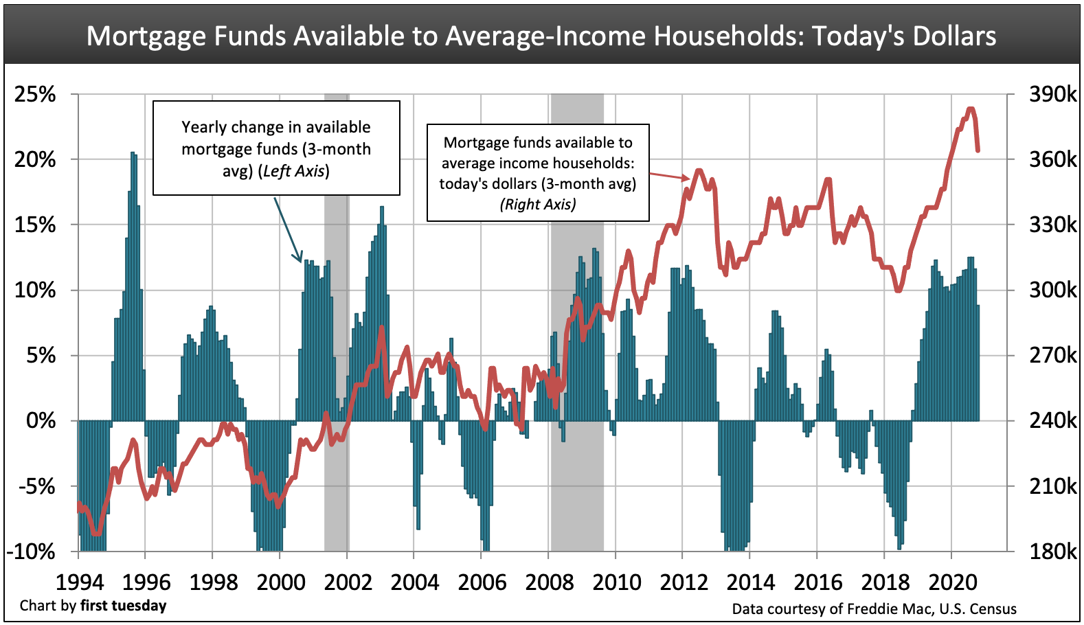
Chart update 04/04/21
| Mar 2021 | Mar 2020 | Mar 2019 | |
| Buyer purchasing power index (1-year percent change in available mortgage funds) | +5.2 | +8.9 | +1.2 |
Chart 2
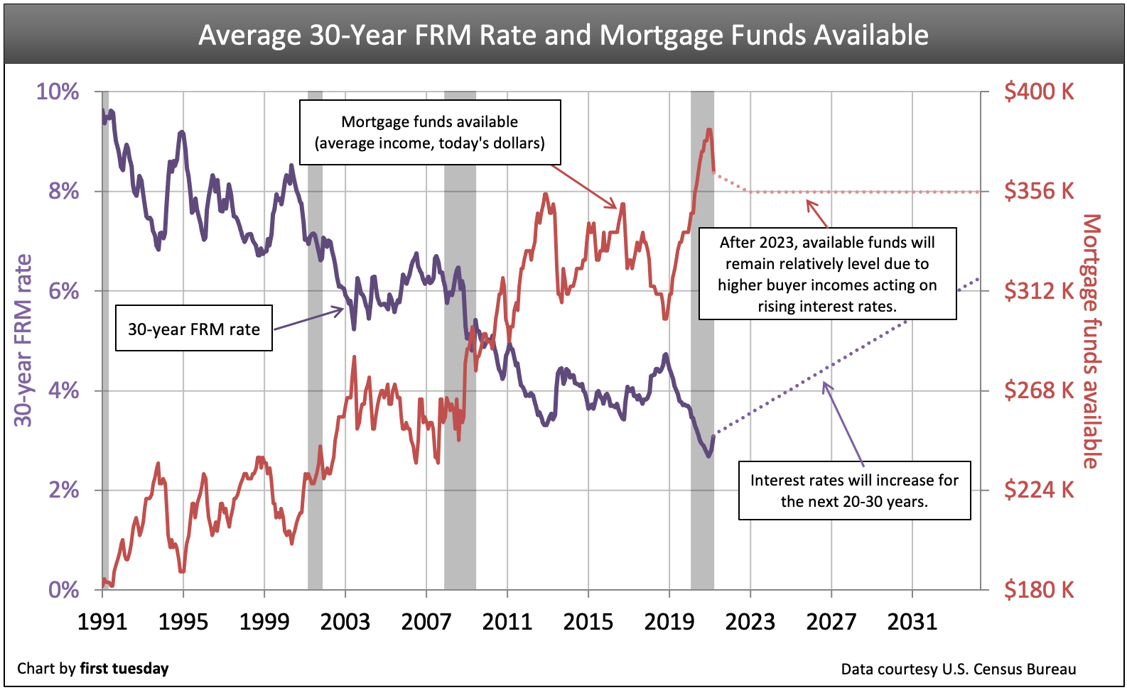
Chart update 04/04/21
| Mar 2021 | Mar 2020 | Mar 2019 | |
| Average 30-year fixed rate mortgage (FRM) | 3.08% | 3.45% | 4.24% |
| Mortgage funds available based on average income | $364,200 | $346,300 | $318,000 |
Buyer purchasing power determines home prices
Buyer purchasing power is the driving force behind real estate pricing. On one side of the table sits the buyer with money; on the other is the seller with a property. Between them sits the all-powerful lender.
Chart 1 displays the Buyer Purchasing Power Index. This index measures the year-over-year change in the amount of mortgage money available to a buyer based on average household income. It varies based on the interest rate charged for a 30-year fixed rate mortgage (FRM).
An index of zero translates to no year-over-year change in the amount one can borrow.
A positive index number, say 5, means the buyer can borrow 5% more money this year than one year earlier. Indexes are based on today’s average household income.
Finally, a negative index figure translates to a reduced amount of mortgage funds available compared to one year earlier.
Related article:
Press Release: Buyer purchasing power index goes positive as mortgage rates remain low
Chart 2 contrasts the average 30-year FRM rate with the corresponding mortgage funds available, in today’s dollars. Over the past 20 years, interest rates have generally decreased, resulting in more funds available to buyers each year.
FRM rates began to rise significantly in 2018 due to the Federal Reserve’s (the Fed’s) raising of the short-term rate. As a result, lenders adjusted 30-year FRM rates upward in order to maintain their profit margins.
As interest rates increase, buyer purchasing power decreases.
The opposite occurred in 2019, when bond market investors began preparing for the Fed to drop their benchmark interest rates. Due to the anticipation (and eventual realization) of lower short-term rates, average FRM rates decreased through 2019 and 2020, resulting in an increased buyer purchasing power. This higher purchasing power had the effect of buoying home prices, seeing them increase despite flat-to-down home sales volume.
Chart 2 displays how falling interest rates increased the mortgage funds available for buyers over the past 20 years. As interest rates rise over the next 20 years, this principle will work in reverse. Mortgage funds available to buyers will decrease. However, the astute reader will notice that the amount of available mortgage money, measured in today’s dollars, flat-lines after 2020. Several factors push and pull on buyer purchasing power to create this plateau trend:
- Population growth in California’s urban cores will create economic support for the state’s economy.
- A buoyed economy will lead to higher median incomes, meaning buyers will have more funds to spend.
- As buyers with more money flood the market, home sale prices will increase.
- Increased income will be countered by rising interest rates.
Together, increased income and rising interest rates will level out buyer purchasing power. Read on to learn about how interest rate movements influence pricing. This knowledge will help you counsel your seller and buyer clients to get the most from a sales transaction.
The lender determines the buyer’s loan amount
Each buyer has a maximum price they can pay to purchase property. This maximum price depends on:
- the buyer’s down payment; and
- the mortgage funds they qualify to borrow from a lender.
The amount of mortgage funds a buyer can borrow is based on two factors:
- the buyer’s income, which adjusts annually at the rate of inflation; and
- current mortgage rates, which change constantly.
Lenders know buyers are less likely to default if they allocate no more than 31% of their monthly gross income to their monthly mortgage payment. Accordingly, mortgage lenders generally refuse to lend more money than the buyer can repay at that 31% gross income ratio, amortized over 30 years.
Buyers control the seller’s price
On the other hand, sellers seek the highest possible sales price they can get from a buyer. The sales price of all homes sold within each pricing tier cannot exceed the purchasing power of buyers shopping in that tier.
If all sellers within a tier hold out for above-market prices, buyers for that tier of property will not be able to buy. Thus, buyers control the price sellers will receive, based mostly on loan funds available at current interest rates.
Chart 1 illustrates that sellers have received greater and greater prices over the past 20 years as interest rates dropped. But be alert, this will not be the trend moving out of a zero-bound interest rate condition, experienced until 2015 and again beginning in 2020. Interest rates cannot drop for the next couple of decades. Short-term rates are still near zero — and the Fed will not go negative. Expect rates to rise over the next 30 years (except during recessions).
The maximum amount mortgage lenders will lend a qualified buyer depends on current mortgage rates. As mortgage rates rise, the maximum price a buyer can pay declines since the amount they are able to borrow declines. The static 31% debt-to-income ratio (DTI) is set for buyers needing a mortgage. Going forward, buyer income will change annually based on consumer inflation of 2%-3%. This has been typical for nearly two decades, except during recessions when buyer income usually decreases.
As interest rates rise, the interest portion of monthly payments on new mortgages rises. The result is a reduction in the portion of each payment that goes toward amortizing the loan principal. The smaller the principal loan amount, the less price sellers can get from buyers. It is axiomatic.
Related article:
Reading the charts
The mortgage funds available to a buyer from year to year are depicted by the red line on Chart 1. These amounts are in today’s dollars and are based on the loan amount an average income earner in California qualifies to borrow. Payments are set at 31% of gross income (before withholdings).
Both charts are in today’s dollars of income. Thus, what appears is a purchasing power change of roughly $100,000 over the past 20 years — due solely to interest rate reductions.
As of 2016, the average monthly income in California was $5,645. At 31% of this monthly income, the maximum mortgage payment the average person can qualify for is $1,750. This amount includes any interest the buyer pays to the bank. Thus, the money available to pay for a new home (the principal payment) changes from week to week with rising and falling interest rates. The rates used on the charts are for a 30-year FRM.
The yearly change in available mortgage funds (green bar) on Chart 1 depicts the percentage change in mortgage funds available compared to one year earlier. Mortgage funds change as interest rates rise and fall. The higher the green bar, the higher the loan amount a buyer will qualify for compared to the previous year using today’s pay. Conversely, the lower the green bar, the fewer mortgage funds can be borrowed by a buyer compared to one year earlier.
Related article:
Chart 1: Historical examples
The significance of the one-year rate differential can be seen on Chart 1 in the following historical examples:
- 2003: Mortgage rates were too low during this period, an aberration in rates due to the Fed’s overreaction to 9/11 attacks. The Fed kept rates low, instead of allowing the 2001 recession to work its pricing magic. Due to lower rates, buyers were able to borrow much more than they could a year or two earlier.
- This led to a spike in buyer purchasing power. Sellers and their agents recognized the increase in mortgage amounts buyers qualified to borrow, and began demanding higher prices. The financial accelerator of excess loans from all types of lenders artificially drove up the price of collateral — homes. Lenders foolishly accepted that condition.
- 2004 and beginning of 2005: FRM rates flattened, causing buyer purchasing power to stabilize. However, property prices were rising. To compensate for this mixed price/lending condition, lenders, buyers and speculators resorted to adjustable rate mortgages (ARMs).
- ARMs allow lenders to mask the amount of future payments with low up-front rates, called teaser rates. With ARMs, the borrower qualifies for greater loan amounts. However, when those teaser rates adjust upwards, the borrower cannot repay at the higher interest rate.
- End of 2005: Sales volume reached its peak while prices continued to rise. The diminishing numbers of buyers turned to option ARMs and alternative A-paper mortgages (Alt-As), also called liar loans, to meet the prices sought by sellers.
- 2006: Sales prices peaked early in the year. Home prices declined from their artificially inflated status. Buyers and their agents began setting prices by applying fundamentals related to the real world.
- These fundamentals factored in the replacement cost of land and improvements, and the income approach for setting value. As prices declined, speculators temporarily disappeared from the market, except to dump property and recover cash.
- 2009: The Fed lowered interest rates essentially to zero. The rise in buyer purchasing power seen in 2009 produced the classic dead cat bounce inherent in all recessionary drops. Due to the Great Recession and financial crisis, mortgage rates were dramatically lowered by the lender of last resort — the Fed.
- This Fed activity provided all the mortgage financing needed by buyers with down payments as little as 3.5%. Unfortunately, reduced rates and down payment amounts also attracted troublesome speculators and flippers. All this again drove prices of low-tier housing up to unsustainable levels going into 2010.
- The FHA contributed to this mini-frenzy by waiving the 90-day investor holding period through the end of 2014. Flipper activity increased dramatically in 2012-2013, driving prices up wildly at the expense of the seller and the buyer.
- 2016. The Fed began to increase its benchmark short-term rate, the effects rippling throughout the market. Adjustable rate mortgages (ARMs) inched up immediately, but FRM rates were more slow to rise due to excess bond market investment.
- 2018. The Fed’s work to increase interest rates begins to trickle over into FRMs. The average 30-year FRM rate will continue to rise in 2018 and the years following.
- 2019-2020. The economy prepares for recession, bringing FRM interest rates down to induce more borrowing. Buyer purchasing power briefly rises and remains flat.
Buyer purchasing power past its cyclical peak today
In a transaction contingent on financing, the buyer’s gross income acts as a fulcrum between the seller and the mortgage lender. Sellers and lenders seesaw up and down in response to mortgage rate changes. Thus, lenders (and the bond market rates) control movement in the seesaw of pricing — not sellers, not buyers.
As lenders lend more to the same type of buyer, sellers demand a higher price from those potential buyers. However, when rates rise, lenders lend less to the same buyers. This lesser loan amount effectively pulls money from the seller in a shift of wealth to the lender.
While this rise in rates benefits the lender, it forces the seller to drop the price. The buyer can do nothing, as they are a prisoner of their income level. Implicitly and eventually, the seller adjusts the asking price to the amount buyers can pay.
Little rate changes make a big difference
Consider a buyer whose gross annual income ($60,190) allows them to make a monthly payment of $1,555.
The $1,555 monthly payment qualifies them for the following loan amounts on an FRM:
| 4%: $325,800 |
| 4.5%: $306,900 |
| 5%: $289,700 |
| 5.5%: $273,800 |
| 6%: $259,400 |
| 6.5%: $246,000 |
If the interest rate fluctuates so much as half a percentage point, the loan amount changes by thousands. All buyers are subject to the same relative reduction in their mortgages on a rate increase. Thus, sellers as a whole must accept a lesser price if they are to sell at the same sales pace that existed before the rate hike.
Other factors weigh in to change the dynamics of this formula. Sellers, by nature, are culturally susceptible to the age-old real estate phenomenon of sticky prices during recessionary periods. Sellers generally are uninformed about pricing properties in the real estate market. Instead, they believe that they should get more for their property than the neighbor did down the street, whether it sold last year or the year before.
This sticky price phenomenon leads to a seller’s delayed response in properly pricing their property to keep pace with the market. As a result, when mortgage rates rise, the real estate market moves toward a stand still.
Here’s an example:
Consider a buyer who is interested in acquiring a particular home. A year earlier, the buyer qualified to borrow sufficient funds to pay the seller’s price. However, mortgage rates have risen and the buyer is now unable to borrow the same amount of money.
Unsurprisingly, the property the buyer was able to buy just a few months ago is now out of reach due to the interest rate change. The buyer now qualifies to purchase the property at a lower price.
However, as is usually the case, the buyer is not interested in purchasing a lesser property than the one they once were qualified to buy. Buyers will rarely downgrade. If they previously qualified for a mortgage large enough to purchase one home, they tend not to purchase a lower-grade home. They will instead wait until prices or interest rates drop.
Interest rates will rise during the next several decades. In turn, seller’s prices will have to drop, if they are asking more than the equivalent rise in annual consumer inflation.
The agent’s initial solution for keeping their sales volume from dropping is to change the seller’s price to accommodate the mortgage rate change. If not, buyers and sellers will stand still with no ability to make a deal.
The buyer’s position is static as with a fulcrum. The maximum price a buyer can pay for a property is dictated by 31% of their gross income. In turn, the lender’s mortgage rate is controlled by the bond market which dictates lender rates. So who has to give? Buyers can’t, lenders won’t. So sellers must ask the “going price” if their intention is to sell in the current market.
The seller must adjust their price expectations, or exit the market.
Understanding the trends in mortgage rates and the purchasing power of a buyer’s gross income is key. The fulcrum (the buyer’s gross income) currently sits between the lender’s rates and the seller’s price. Agents can intelligently advise their sellers not to sit idly by, unable to locate a buyer due to unrealistic pricing.


Nice post. I was checking constantly this blog and I am
impressed! Very useful information particularly the last part :
) I care for such info a lot. I was looking for this certain information for a long time.
Thank you and good luck.
Helpful info. Lucky me I found your website unintentionally, and I’m shocked why this accident didn’t took place earlier!
I bookmarked it.
With the increase in taxes in California, forward looking agents may have to focus on a downturn instead of an uptick. Listings for expensive homes will probably rise but be much harder to sell. Low priced homes may sell if interest rates were to remain low. However, you can only print so much money before inflation drives the cost of funds higher. Therefore, unless there is a change in policy with the current administration, tax and spend is going to create a real estate nightmare.
I agree with everyone that this is a great site, but I have to take exception to some of the material in this post. Primarily, the tone that certain predictions are stated as if they were facts is misleading. For example:
■Population growth in California’s urban cores will create economic support for the state’s economy.
■A buoyed economy will lead to higher median incomes, meaning buyers will have more funds to spend.
■As buyers with more money flood the market, home sale prices will increase.
■Increased income will be countered by rising interest rates.
In particular, I believe points 2 & 3 are highly speculative and could prove to be disastrously wrong.
I agree with Jeffrey above I have been an agent and broker many years and this information from First Tuesday is the best.
This is a great newsletter. Their continuing education classes are some of the toughest out there, but they make you a better agent.
Hi. I was wondering if you have internet capability to take the National Loan Officer education for California and Nevada Loan Officer exam licensing.
Margaret Munoz,
I have been a Realtor/Broker for over 35 years (Addison Realty & Property Management, Ventura, CA.) , closed hundreds of escrows and I find “First Tuesday Magazine” to be one of the most informative connections to what is happening in real estate today.